Recently, we covered basic concepts of time series data and decomposition analysis. We started talking about common patterns of time series data, like trend, season, and cycle. Then, we described how to explore these patterns using classic decomposition methods. Following that, it’s now time to apply that knowledge to a practical algorithm. In this piece, we provide an overview of Exponential Smoothing Methods.
What Are Exponential Smoothing Methods?
Exponential Smoothing Methods are a family of forecasting models. They use weighted averages of past observations to forecast new values. The idea is to give more importance to recent values in the series. Thus, as observations get older in time, the importance of these values get exponentially smaller.
Exponential Smoothing Methods combine Error, Trend, and Seasonal components in a smoothing calculation. Each term can be combined either additively, multiplicatively, or be left out of the model. These three terms (Error, Trend, and Season) are referred to as ETS.
Exponential Smoothing Methods can be defined in terms of an ETS framework, in which the components are calculated in a smoothing fashion.
As we can see, combining Error, Trend, and Season in at least three different ways gives us a lot of combinations. Let’s consider some examples.
Using the taxonomy described at Forecasting: Principal and Practice, the three main components can be defined as:
- Error: E
- Trend: T
- Season: S
Moreover, each term can be used in the following ways:
- Additive: A
- Multiplicative: M
- None: N (Not included)
Thus, a method with additive error, no trend and no seasonality would be referred to ETS(A,N,N) — which is also known as Simple Exponential Smoothing with an additive error.
Following the same reasoning, we have:
- ETS(M,N,N): Simple exponential smoothing with multiplicative errors.
- ETS(A,A,N): Holt’s linear method with additive errors.
- ETS(M,A,N): Holt’s linear method with multiplicative errors.
But how can we decide how to best apply each of these components using the ETS framework?
Time Series Decomposition Plot
Analyzing whether time series components exhibit additive or multiplicative behavior rests in the ability to identify patterns like trend, season, and error. And that’s the idea behind time series decomposition.
As we saw in our last article about the subject, the goal of time series decomposition is to separate the original signal into three main patterns.
- The Trend
- The Season
- The Error (also known as residuals or remainder)
The trend indicates the general behavior of the time series. It represents the long-term pattern of the data — its tendency.
The seasonal component displays the variations related to calendar events. Lastly, the error component explains what the season and trend components do not. The error is the difference between the original data and the combination of trend and seasonality. Thus, if we combine all three components, we get the original data back.
Usually, decomposition methods display all this information in a decomposition plot.
 Analyzing a Time Series Decomposition Plot is one of the best ways to figure out how to apply the time series components in an ETS model.
Time Series Decomposition Analysis
Quick recap! Using the ETS framework, each component — trend, season, and error — can be applied either additively or multiplicatively. We can also leave one or more of these components out of the model if necessary.
Let’s now consider some ways to identify additive or multiplicative behavior in time series components.
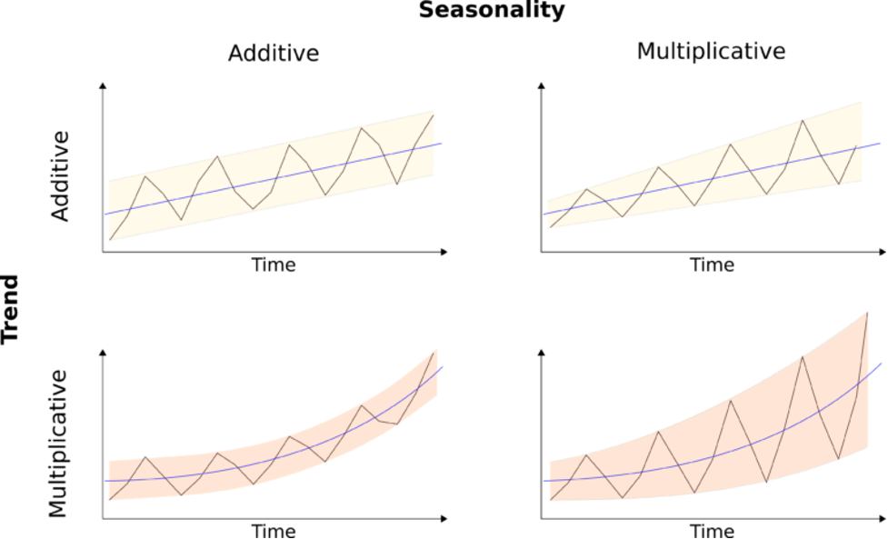
In general, additive terms show linear or constant behavior.
If the trend component increases or decreases linearly, or close to it, we say it has an additive pattern. On the other hand, if the trend shows an exponential variation, either positive or negative, then it has a multiplicative behavior.
The Season component follows a similar pattern. However, here we are more interested in variations of magnitude. Seasonal patterns always occur at regular intervals. When the magnitude of the seasonal swings remains constant, it has an additive behavior. Otherwise, if magnitude changes over time, it has multiplicative behavior.
The same applies to the Error component. If the magnitude varies over time, we also apply it multiplicatively.
Let’s now jump to a practical example. Consider the time series for Gas Consumption in the UK. This dataset contains 108 quarterly-spaced point values from 1960 to 1986.
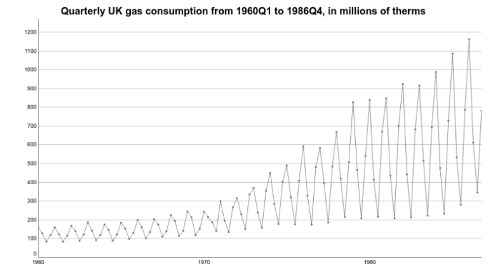
Before any decomposition, we can already extract some insights from the time series plot. First, the general trend is positive. It shows a general positive gradient throughout the data.
Seasonal variations are also very strong. Gas consumption for the first and last quarters are higher throughout the series. Also, note that the magnitude of gas consumption increases over time. The latter indicates a multiplicative seasonal term.
Now, take a look at the time series decomposition plot.
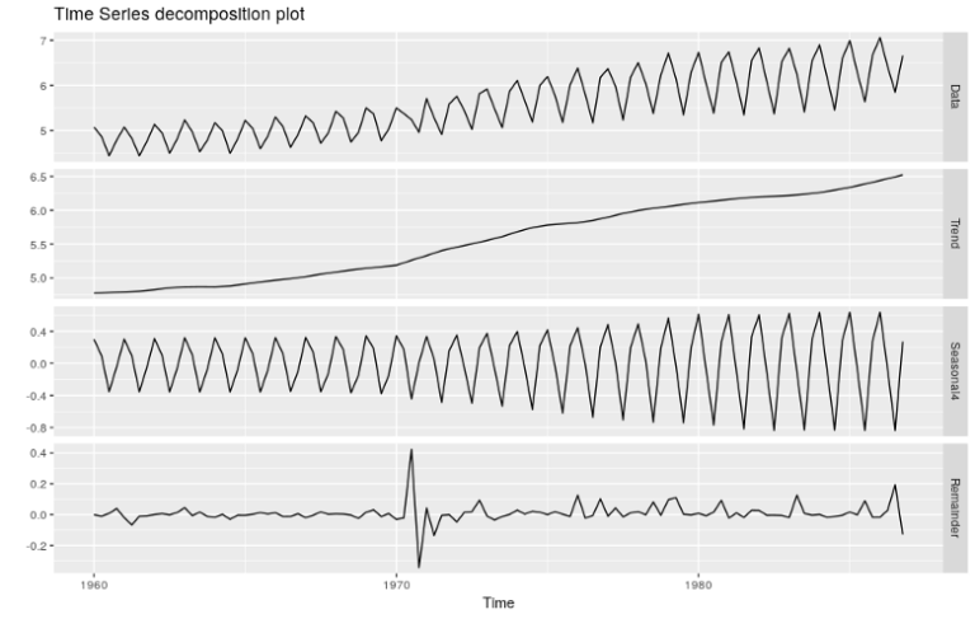
The plot above shows an STL decomposition.
STL only performs additive decomposition. However, based on our knowledge so far, we can also find patterns that might indicate multiplicative terms. The decomposition plot shows the original data on top, followed by the Trend, Seasonal, and Error (Remainder) components.
As we expected, the Trend shows additive behavior — it grows somewhat linearly.
Note that the seasonal variations are not constant over time. We can see that the magnitude of the seasonal fluctuations increases throughout the time series.
Lastly, the Remainder component displays a change in variance as the time series moves along. Thus, both, Seasonal and Error components should be applied as a multiplicative term.
Thus, we can define our model as ETS(M,A,M).
- Multiplicative Error
- Additive Trend
- Multiplicative Seasonality
You can see the smoothing equations for this method here.
Let’s take the years from 1960 to 1984 as a training set and reserve the last two years for testing. Now, we can fit an ETS(M,A,M) using the training set and perform forecasting for the next two years. Check the results below.

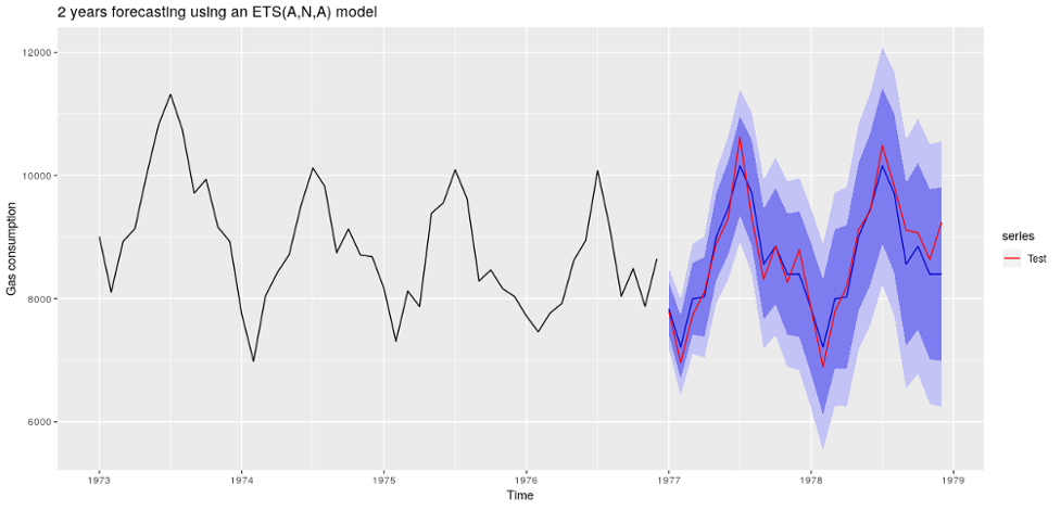
The test data is shown in red, and predictions plus confidence interval are in blue. Note how the forecasting confidence variations increase over time. That’s a normal pattern that reflects the model uncertainty to predict values further in the future.
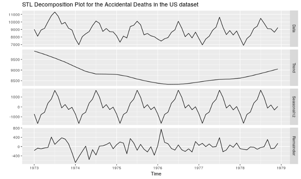
Let’s take a different example. The next time series shows monthly data about Accidental Deaths in the US from 1973 to 1978.
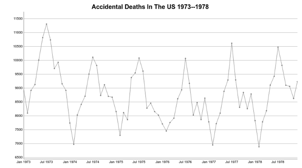
Like in the previous example, seasonal variations are very strong. July is the deadliest month while February exhibits the least occurrences. Also, this pattern repeats year after year.
What’s different from the last example, though, is the fact that seasonality does not display significant changes in variance. If the magnitude of seasonal variations exhibits a constant behavior over time, we can apply it as an additive term. Besides, note that the data does not show a clear upward or downward trend. Have a look at this decomposition plot.
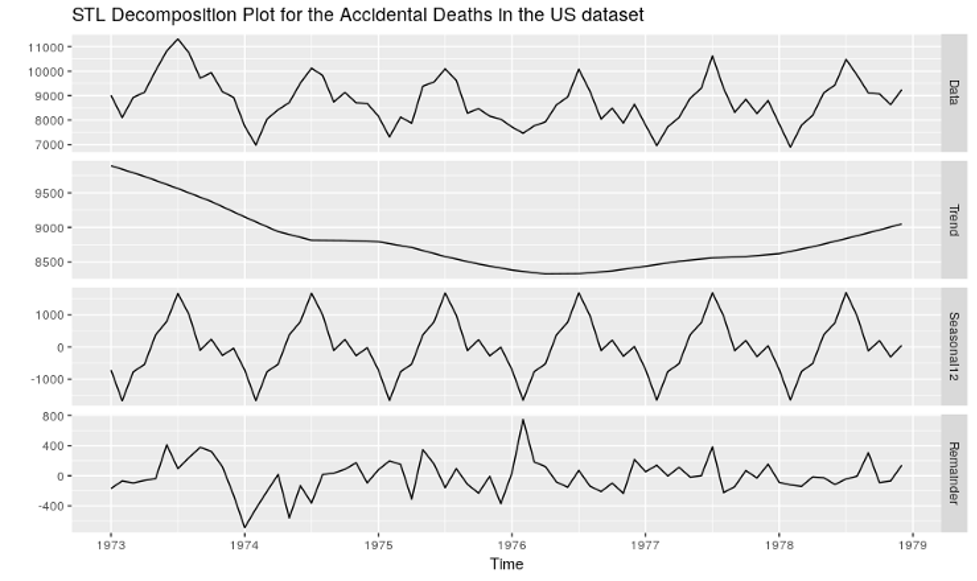
The trend seems to show a down-to-up pattern. If we overlay the trend on top of the time series, it looks very close to a horizontal pattern. Then, it seems reasonable to leave it out of the model.
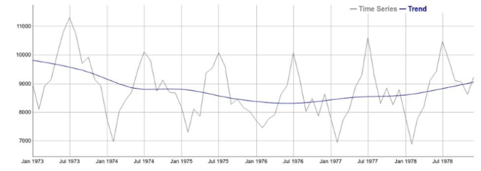
As we expected, the magnitude of the seasonal variations looks very much constant. Moreover, the Error term does not show significant variations as well. Thus, it seems reasonable to apply both Season and Error as additive terms to the model. This gives us an ETS(A,N,A) — Additive Error, No Trend, and Additive Seasonality.
Reserving the last two years for testing, the resulting forecast for ETS(A,N,A) looks like this:
Conclusion
These are some key points to take from this piece.
- Exponential Smoothing Methods are a family of classic forecasting algorithms. They work well when the time series shows a clear trend and/or seasonal behavior.
- Exponential Smoothing Methods combine Error, Trend, and Season. We can apply each of these components either additively or multiplicatively.
- Time series decomposition is one of the best ways to find patterns of Trend, Season, and/or Error. A decomposition plot usually shows each component as a separate subplot.
- If the trend shows a linearly upward or downward tendency, we apply it additively. If it varies exponentially, it’s multiplicative.
- If the magnitude of the seasonal patterns changes linearly, we can apply it additively. If the magnitude evolves exponentially, it is multiplicative.
Acknowledgment
This article is a contribution of many Encora professionals: Thalles Silva, Bruno Schionato, Diego Domingos, Fernando Moraes, Gustavo Rozato, Isac Souza, Marcelo Mergulhão and Marciano Nardi.
About Encora
Fast-growing tech companies partner with Encora to outsource product development and drive growth. Contact us to learn more about our software engineering capabilities.